library(barrks)
library(tidyverse)
library(terra)


# function to unify the appearance of raster plots
my_rst_plot <- function(rst, ...) {
  plot(rst, mar = c(0.2, 0.1, 2, 5),
       axes = FALSE, box = TRUE, nr = 1,
       cex.main = 1.9, plg = list(cex = 1.8), ...)
}
Calculate phenology
In this vignette, the sample data delivered with barrks
is used to calculate the phenology with all models available in the
package. Note that the daylength threshold for diapause initiation of
the Jönsson model is adapted to Central Europe according to Baier, Pennerstorfer, and Schopf (2007).
data <- barrks_data()

# calculate phenology
phenos <- list('phenips-clim' = phenology('phenips-clim', data),
               'phenips' = phenology('phenips', data),
               'rity' = phenology('rity', data),
               'lange' = phenology('lange', data),
               # customize the Jönsson model for Central Europe
               'joensson' = phenology(model('joensson', daylength_dia = 14.5), data),
               'bso' = bso_phenology(.data = data) %>% bso_translate_phenology(),
               'chapy' = phenology('chapy', data))
Spatial outputs
barrks provides different functions to examine the
results of the phenology calculations. This section describes the
application of the basic functions that return spatial outputs.
Day-of-year-rasters
The onset of infestation, initiation of diapause and the
frost-induced mortality are described as the corresponding day of year.
That data can be attained via get_onset_rst(),
get_diapause_rst() or get_mortality_rst(). As
some models have not all submodels implemented and
terra::panel() does not allow adding empty rasters, a
workaround-function is defined to plot the the respective submodel
outputs. Additionally, it draws the borders of the area of interest.
plot_doy_panel <- function(x) {

  aoi <- as.polygons(data[[1]][[1]] * 0)

  draw_aoi_borders <- function(i) {

    if(empty[i]) polys(aoi, lwd = 2, col = 'white')
    else polys(aoi, lwd = 2)
  }

  # replace NULL by a raster with values in the overall range to not affect the legend
  # the raster will be overplotted by `draw_aoi_borders()`
  rst_tmp <- data[[1]][[1]] * 0 + min(minmax(rast(discard(x, is.null)))[1,])
  empty <- map_lgl(x, \(y) is.null(y))
  walk(which(empty), \(i) x[[i]] <<- rst_tmp)

  panel(rast(x),
        names(x),
        col = viridisLite::viridis(100, direction = -1),
        axes = FALSE,
        box = TRUE,
        loc.main = 'topright',
        fun = draw_aoi_borders,
        cex.main = 1.9,
        plg = list(cex = 1.8))
}

plot_doy_panel(map(phenos, \(p) get_onset_rst(p)))
plot_doy_panel(map(phenos, \(p) get_diapause_rst(p)))
plot_doy_panel(map(phenos, \(p) get_mortality_rst(p)[[1]]))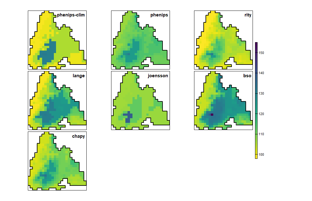
Day of year when the infestation begins
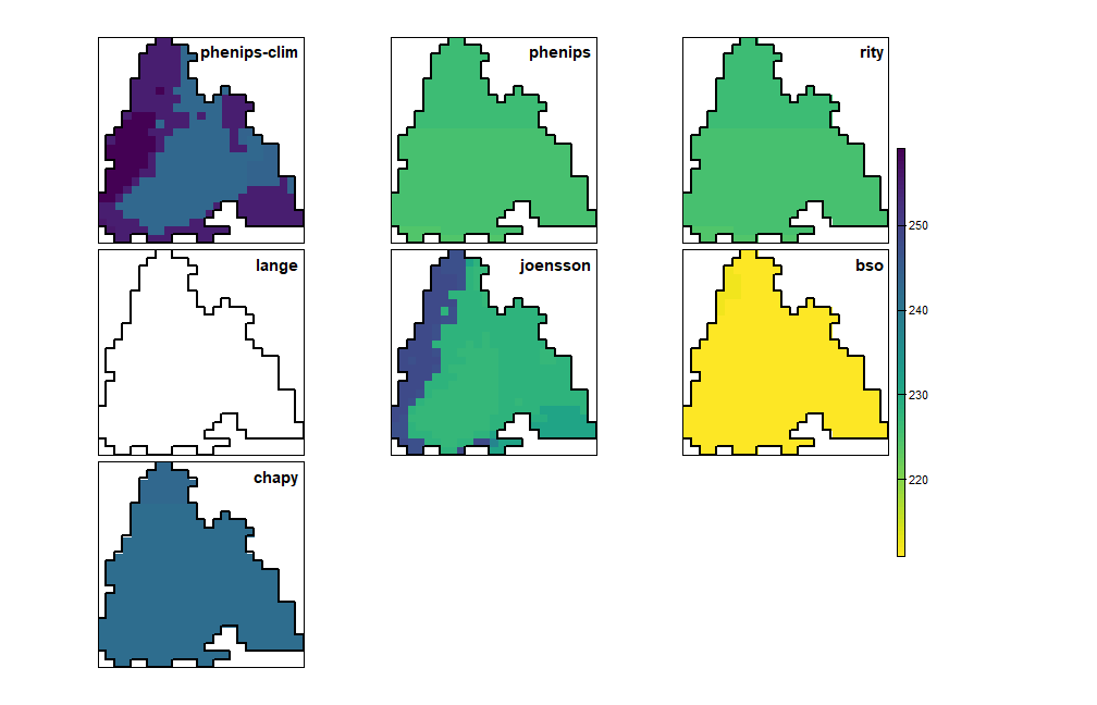
Day of year when the diapause begins (in white cells no diapause was induced)
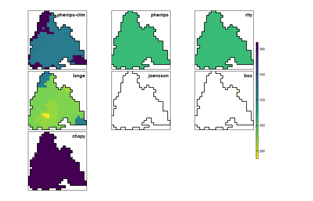
Day of year of the first frost-induced mortality event in autumn/winter (in white cells no mortality occured)
Generations
To get an overview of the establishment of generations, it is
possible to plot the prevailing generations on different dates using
get_generations_rst() and my_rst_plot().
# dates to plot
dates <- c('2015-04-15', '2015-06-15', '2015-08-15', '2015-10-15')

# walk through all phenology models
walk(names(phenos), \(key) {

  p <- phenos[[key]]

  # plot generations of current model
  get_generations_rst(p, dates) %>% my_rst_plot(main = paste0(key, '-', dates))
})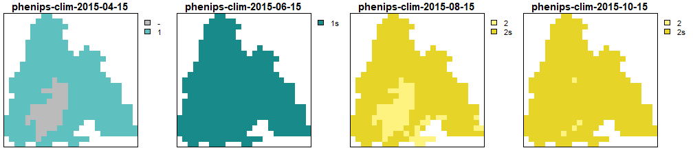
Generations calculated by PHENIPS-Clim
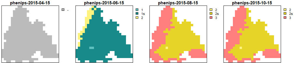
Generations calculated by PHENIPS
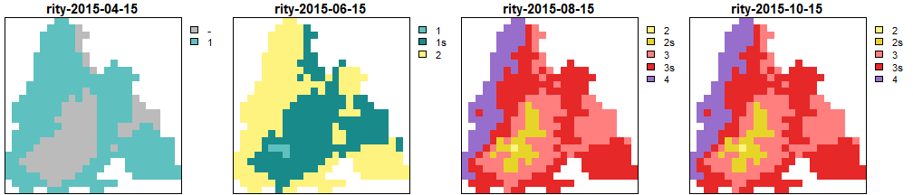
Generations calculated by RITY
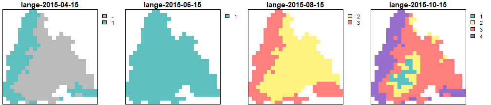
Generations calculated by the Lange model
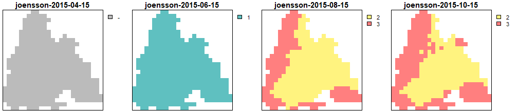
Generations calculated by the Jönsson model
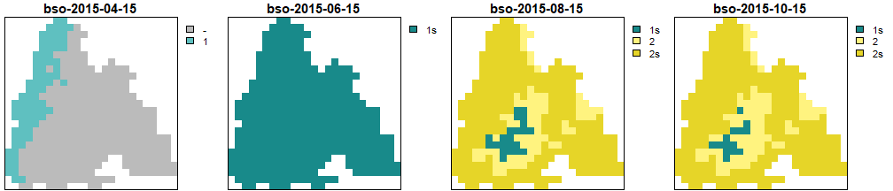
Generations calculated by BSO
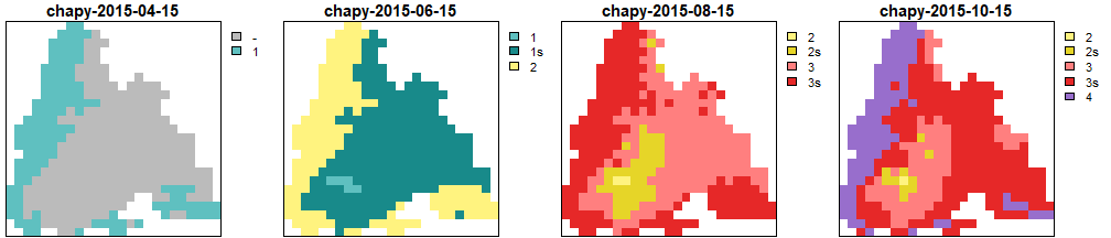
Generations calculated by CHAPY
Stationwise outputs
To plot the development diagrams of particular raster cells, stations
can be defined by specifying their cell numbers. To get the stations’
coordinates, terra::xyFromCell can be used.
# plot the locations of the stations

rst_aoi <- data[[1]][[1]] * 0
stations <- stations_create(c('station 1', 'station 2'), c(234 345))
station_coords <- vect(xyFromCell(rst_aoi, stations_cells(stations)))

plot(rst_aoi,  col = '#AAAAAA', legend = FALSE, axes = FALSE, box = TRUE)
plot(station_coords, col = 'red', pch = 4, add = TRUE)
text(station_coords, names(stations), col = 'black', pos = 2)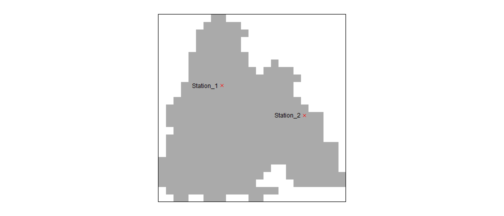
Stations map
The stations should be passed to
plot_development_diagram() to get the desired plots. Here,
only the models PHENIPS-Clim and PHENIPS are plotted to reduce the
complexity of the diagrams.
# plot the development diagrams

limits <- as.Date(c('2015-04-01', '2015-12-31'))

models <- c('phenips-clim', 'phenips')

walk(1:length(stations), \(i) {
  plot_development_diagram(phenos[models],
                           stations[i],
                           .lty = 1:length(models),
                           .group = FALSE,
                           xlim = limits)
})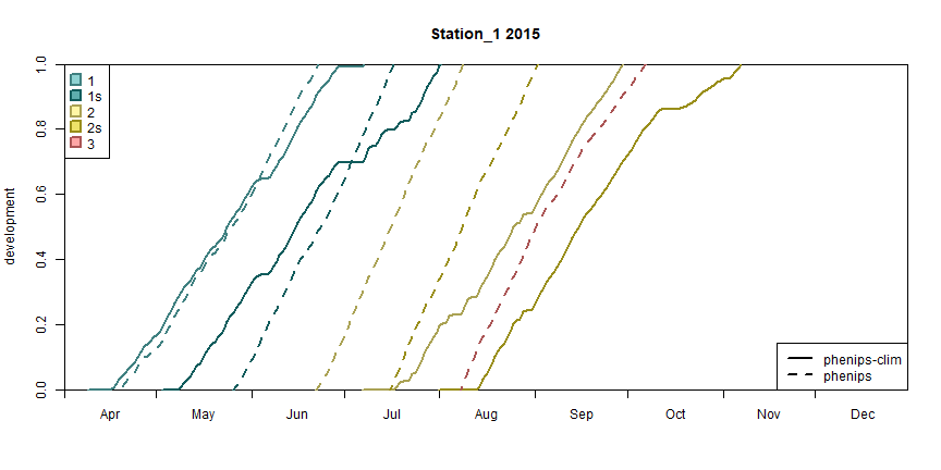
Development diagram for station 1
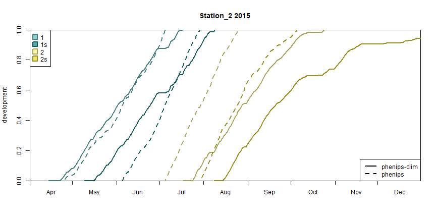
Development diagram for station 2